The problem
A person is feeling sick and decides to take a rapid Covid test. Unfortunately, the test comes back positive.

A positive test result
The test is positive, but how certain can the person be that they are truly infected with Covid, i.e., how certain can they be that the test result is accurate? The same question could be asked if the test were negative: How certain is it in this case that the person is truly not infected with Covid?
The problem
What is the probability that a person with a positive Covid test is truly infected? What is the probability that a person with a negative Covid test is truly healthy?
First, we take a look at the package insert of the rapid test in the hope of finding answers to our questions.
The package insert of a commercial Covid rapid test
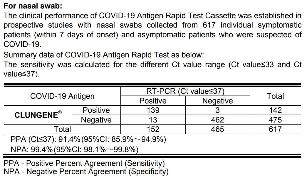
Confusion matrix of the rapid test
| Person sick | Person healthy | Total | |
|---|---|---|---|
| Test positive | 139 | 3 | 142 |
| Test negative | 13 | 462 | 475 |
| Total | 152 | 465 | 617 |
Let’s try to decipher the information. Apparently, a study was conducted in which samples were taken from individuals. These samples were subjected to an RT-PCR test and a rapid test of the CLUNGENE brand via nasal swab, and the results of both tests were compared for each person.
In this study, we are only interested in the accuracy of the rapid test. To do this, we assume that the result of the RT-PCR test is exact and that we know whether a person is infected with Covid or not. We then check whether the rapid test correctly identifies the health status of the individuals or not. From here on, we will refer to the Covid rapid test simply as test.
When we evaluate the result of such a test, we can first determine that we are dealing with four possible outcomes:
- The person is sick and the test is positive.
- The person is sick and the test is negative.
- The person is healthy and the test is positive.
- The person is healthy and the test is negative.
This can be presented as a table:
| Person sick | Person healthy | |
|---|---|---|
| Test positive | true positive | false positive |
| Test negative | false negative | true negative |
This table representation is called a confusion matrix.
Below the confusion matrix in the package insert, we find two percentage values: PPA and NPA. These were calculated from the values in the table and are quality measures for medical tests:
PPA stands for positive percent agreement or true positive rate, or sensitivity. The value indicates how many percent of confirmed positive Covid cases are correctly identified as positive by the test. In our test, it is on average 91.4%.
NPA stands for negative percent agreement or true negative rate, or specificity. The value indicates how many percent of confirmed negative Covid cases are correctly identified as negative by the test. In our test, it is on average 99.4%.
Why do test accuracy, sensitivity, and specificity not answer our actual question, which we see in the summary at the top right? We will look at this on the following page.
Analysis
To formalize the problem, we represent the procedure in the study as a tree diagram, which will later help us answer the actual question. We know who is healthy and who is sick and check for each group of people how the test turns out:

Tree diagram with events
We will first define two events and their negation to help us do the number work. They correspond to the possibilities mentioned above.
- \(S\): Person sick,
- \(\overline S\): person healthy,
- \(T\): test positive,
- \(\overline T\): test negative.
Definition of the events
- \(S\): Person sick and \(\overline S\): person healthy,
- \(T\): test positive and \(\overline T\): test negative.
We can transfer these events to a tree diagram, together with the associated probabilities \(P\):
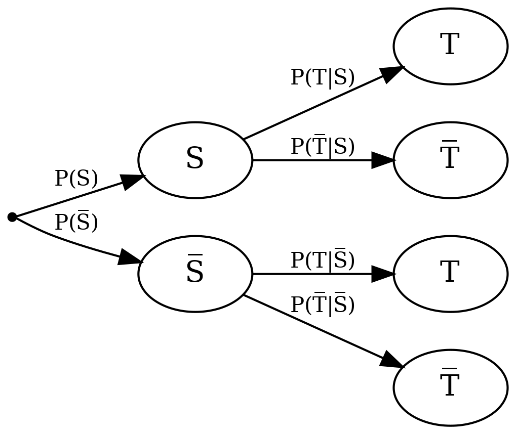
Tree diagram with events and their probabilities
As formulated in the question, we want to know the probability that a person is actually sick if the test is positive. This can be formulated using the above-defined events as conditional probability – the probability that a person is sick, given that the test is positive: \(P(S \mid T)\). This probability is also called positive predictive value, but it does not appear in the above tree diagram. There, the events \(S\) and \(T\) are reversed as in \(P(T \mid S)\).
\(P(T \mid S)\) is called sensitivity and is a quality measure for a test, as we have already seen in the package insert. Sensitivity indicates how high the probability is that the test shows a positive result for a person who is actually sick and is therefore also called true positive rate.
To calculate the actually sought positive predictive value, i.e., the conditional probability \(P(S \mid T)\), we can use Bayes’ Theorem:
\[ P(S \mid T) = \frac{P(T \mid S) P(S)}{P(T)}. \]
So what we need to calculate \(P(S \mid T)\) are three probabilities: \(P(S)\), \(P(T \mid S)\), and \(P(T)\).
Definition of conditional probabilities
\(P(S \mid T)\) – Probability that a person is actually sick, given that the test is positive.
Bayes’ Theorem
\[ P(S \mid T) = \frac{P(T \mid S) P(S)}{P(T)}. \]
\(P(S)\) indicates how high the probability is generally to be infected with Covid at this time – completely independent of a test result. This value is also called prevalence. We can never know this probability exactly, but we can take an estimated value that corresponds to the proportion of currently infected people in Germany. Let’s first set \(P(S) = 0.2\%\). This is roughly the prevalence during the first wave of Covid in spring 2020 in Germany.
One might also come up with the idea of reading \(P(S)\) from the study in the package insert, but this is not sensible in most cases: the study that led to the results in the package insert precisely examines how well the test works in sick people, so that people with proven Covid infection were specifically tested. This cannot be spoken of as a cross-section of the population.
Definition of conditional probabilities
\(P(T \mid S)\) – Probability that a test shows a positive result, given that the person is actually sick (sensitivity).
The probability \(P(T \mid S)\) is already given in the package insert as sensitivity.
Finally, we are missing \(P(T)\): the probability that a person – whether sick or healthy – receives a positive test result. Here, the law of total probability helps us, which allows us to add the probabilities for the two possibilities that lead to positive tests (person sick and person healthy), since they exclude each other:

Tree diagram with both possibilities that lead to positive tests
Thus, we get
\[ P(T) = P(T \mid S) P(S) + P(T \mid \overline S) P(\overline S), \]
and thus
\[ P(S \mid T) = \frac{P(T \mid S) P(S)}{P(T)} = \frac{P(T \mid S) P(S)}{P(T \mid S) P(S) + P(T \mid \overline S) P(\overline S)}. \]
However, this brings us two new problems: we need \(P(T \mid \overline S)\) and \(P(\overline S)\). Fortunately, we can calculate both via the probability of complementary events. Thus, \(P(\overline S)\) (the general probability of not being sick) is easy to calculate, because we already know \(P(S)\) (the general probability of being sick, estimated using prevalence): \(P(\overline S) = 100\% - P(S) = 99.8\%\).
Finally, we are still missing \(P(T \mid \overline S)\): the probability of having a positive test result when one is actually healthy (a false positive result). Here, another quality measure for tests helps us: the specificity, also called true negative rate. It gives us the probability that a person receives a negative test result when they are actually healthy, so \(P(\overline T | \overline S)\). The specificity is often printed in the package insert of rapid tests, as we have already seen. As we can see in the tree diagram, \(P(\overline T | \overline S)\) is complementary to \(P(T | \overline S)\) and thus \(P(T | \overline S) = 100\% - P(\overline T | \overline S)\).
Bayes’ Theorem
\[\begin{align} P(S \mid T) &= \frac{P(T \mid S) P(S)}{P(T)} \\ &= \frac{P(T \mid S) P(S)}{P(T \mid S) P(S) + P(T \mid \overline S) P(\overline S)}. \end{align}\]
Definition of conditional probabilities
\(P(\overline T \mid \overline S)\) – Probability that a test shows a negative result, given that the person is actually healthy (specificity).
Calculation
To calculate how high the probability is that a person is actually sick if they receive a positive test result from our considered rapid test, we note the sensitivity and specificity from the package insert again:
- Sensitivity: \(P(T \mid S) = 91.4\%\),
- and specificity: \(P(\overline T \mid \overline S) = 99.4\%\).
For the prevalence we had assumed \(P(S) = 0.2\%\).
With this, we can plug the values into the formula and get:
\[\begin{align} P(S \mid T) &= \frac{P(T \mid S) P(S)}{P(T \mid S) P(S) + P(T \mid \overline S) P(\overline S)} \\[10pt] &= \frac{P(T \mid S) P(S)}{P(T \mid S) P(S) + (1 - P(\overline T \mid \overline S)) (1 - P(S))} \\[10pt] &= \frac{0.914 \cdot 0.002}{0.914 \cdot 0.002 + (1 - 0.994) \cdot (1 - 0.002)} \\[10pt] &= 0.2339. \end{align}\]
Interpretation
The probability that a person with a positive rapid test is actually sick (positive predictive value) is only about \(23\%\). This is actually not a particularly high probability and at first glance surprising, because both sensitivity and specificity are close to 100% as quality measures in the package insert of the test. On the next page, we will take a closer look at why this is the case.
Quiz tasks
Introduction to code tasks
In this learning application, you will also be given tasks to solve using R code. These tasks involve short code snippets that you should either complete (by replacing placeholders with corresponding code) or write entirely on your own. In most cases, you will generate a final result, which must be the outcome of the last line.
Example task: Determine the mean value of the numbers on a six-sided die. In the code, we have already provided the numbers 1 to 6 in the variable die. Now use an appropriate R function to determine the mean value from these numbers. Replace the placeholder ___ for this purpose.
die <- 1:6
___(die)
die <- 1:6
mean(die)You can calculate the arithmetic mean in R using the function mean().
As you can see, you need to write the code that produces the final result in the last line of the code input.
Code task 1a
In the following code, the confusion matrix confmat is generated with the values from the package insert.
Extend the code so that confmat is expanded by the marginal sums. Use the function addmargins for this purpose.
confmat <- matrix(c(139, 13, 3, 462), ncol = 2)
colnames(confmat) <- c("sick", "healthy")
rownames(confmat) <- c("positive", "negative")
confmat
confmat <- matrix(c(139, 13, 3, 462), ncol = 2)
colnames(confmat) <- c("sick", "healthy")
rownames(confmat) <- c("positive", "negative")
confmat2 <- addmargins(confmat)
confmat2Code task 1b
In the following code, the confusion matrix confmat is generated with the values from the package insert. Calculate \(P(T \mid S) = \frac{P(T, S)}{P(S)}\) directly using confmat. You can access the value in row i and column j by using the syntax confmat[i, j]. You can select the entire row i using confmat[i,] and the entire column j using confmat[,j].
confmat <- matrix(c(139, 13, 3, 462), ncol = 2)
colnames(confmat) <- c("sick", "healthy")
rownames(confmat) <- c("positive", "negative")
confmat
confmat <- matrix(c(139, 13, 3, 462), ncol = 2)
colnames(confmat) <- c("sick", "healthy")
rownames(confmat) <- c("positive", "negative")
confmat[1, 1] / sum(confmat[,1])Select the corresponding value for \(T \cap S\) (positive test and sick) from confmat using confmat[i,j]. Also, calculate the number of people who were proven to be sick as the sum of the “sick” column. You can do this by selecting the column and using the sum() function. Then, divide the count for \(T \cap S\) by the count for \(S\).
The influence of prevalence and test accuracy
Let’s take another look at the calculation of the conditional probability \(P(S \mid T)\):
\[\begin{align} P(S \mid T) &= \frac{P(T \mid S) P(S)}{P(T \mid S) P(S) + P(T \mid \overline S) P(\overline S)} \\[10pt] &= \frac{0.914 \cdot 0.002}{0.914 \cdot 0.002 + 0.006 \cdot 0.998} \\[10pt] &= 0.2339. \end{align}\]
This equation clearly shows the significant influence of prevalence on the overall result: Even with a high sensitivity of the test, the numerator \(P(T \mid S) P(S)\) and thus the overall result become very small when the prevalence is very low. This also makes intuitive sense: If there are very few cases of a disease overall, the probability that a person is actually affected by it, even if the test is positive, is comparatively low. In contrast, the probability is very high that a person is affected by a disease with many cases (i.e., high prevalence) regardless of how well the test performs.
We can also visualize this by plotting \(P(S \mid T)\) as a function of prevalence for fixed sensitivity and specificity:

We see how steeply the curve rises, and starting at a prevalence of 10%, we can really trust a test result with the given sensitivity and specificity. For a lower prevalence, this is less justified, as shown here in more detail:
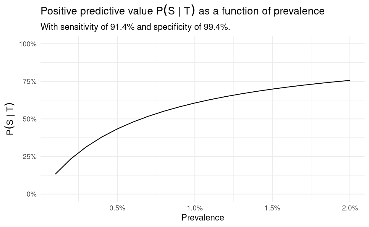
On the other hand, it also demonstrates how important accurate tests are. In the case of low prevalence, specificity plays a particularly important role, as the following graphics illustrate:

By using this interactive graphic, you can illustrate the positive predictive value in relation to the prevalence for self-chosen sensitivity and specificity values:
The specificity \(P(\overline T \mid \overline S)\) has a great influence, because as we have already shown
\[\begin{align} P(S \mid T) &= \frac{P(T \mid S) P(S)}{P(T \mid S) P(S) + P(T \mid \overline S) P(\overline S)} \\[10pt] &= \frac{P(T \mid S) P(S)}{P(T \mid S) P(S) + (1 - P(\overline T \mid \overline S)) P(\overline S)}, \end{align}\]
and since \(P(S)\) is very small, \(P(\overline S)\) is very large and thus the specificity \(P(\overline T \mid \overline S)\) has the “power” over the denominator through the term \((1 - P(\overline T \mid \overline S)) P(\overline S)\). Thus, a high specificity causes a small denominator and therefore a high positive predictive value.
So we see: good tests (notably with high specificity) can make a big difference here especially at the beginning of an outbreak. They allow infections to be detected quite reliably early on, even if the prevalence is still low.
Other parameters and circumstances aside from prevalence and test quality also have a significant influence on the result. In particular, it is important how thoroughly the swab was taken. It is also known that temperature affects the accuracy of Covid rapid tests. So you see that the calculations can become much more complex!
Code task 2a
Analogous to the graphs for the positive predictive value \(P(S \mid T)\), we want to create a graph for the negative predictive value \(P(\overline S \mid \overline T)\). This graph should show the negative predictive value as a function of prevalence and sensitivity.
First, we need a dataframe with a series of prevalence and sensitivity values. Create such a dataframe for all combinations of the prevalence values \(0.1, 0.2, \dots, 0.9\) and the sensitivity values \(0.8, 0.91\) and \(0.99\). You can use the function expand.grid for this. The dataframe should be named npv_param and have the columns prev and sens.
npv_param <- expand.grid(prev = ___,
                         sens = ___)
npv_param
npv_param <- expand.grid(prev = seq(0.1, 0.9, length.out = 9),
sens = c(0.8, 0.91, 0.99))
npv_paramCode task 2b
Next, calculate the negative predictive value \(P(\overline S \mid \overline T)\) for all given parameters and add the result as a column nvw to the dataframe npv_param. Use a fixed specificity of \(99.4\%\).
spec <- 0.994
npv_param$nvw <- ___
npv_param
spec <- 0.994
npv_param$npv <- spec * (1-npv_param$prev) / (spec * (1-npv_param$prev) + (1-npv_param$sens) * npv_param$prev)
npv_paramCode task 2c
Create a plot with ggplot2 that displays the negative predictive value as a function of prevalence. For the three different sensitivity values, three differently colored lines should be displayed.
The resulting plot should look like this:

ggplot(npv_param, aes(___)) +
    ___ +  # "geom_..." für Linienplot
    theme_minimal()
ggplot(npv_param, aes(prev, npv, color = sens, group = sens)) +
geom_line() +
theme_minimal()Data Protection Information
Data Protection Information on Data Collection in the Research Project “MultiLA” according to Art. 13 GDPR
The project “Multimodal Interactive Learning Dashboards with Learning Analytics” (MultiLA) aims to research learning behavior in the provided learning applications. For this purpose, data is collected and processed, which we will now explain.
1. Name and contact details of the responsible party
Hochschule für Technik und Wirtschaft Berlin
Treskowallee 8
10318 Berlin
T: +49.40.42875-0
Represented by the President Praesidentin@HTW-Berlin.de
2. Data Protection Officer
Official Data Protection Officer
Vitali Dick (HiSolutions AG)
datenschutz@htw-berlin.de
Project Manager
Andre Beinrucker
andre.beinrucker@htw-berlin.de
3. Processing of personal data
3.1 Purpose
The processing of personal data serves the purpose of analyzing learning behavior and the use of interactive learning applications within the research project “MultiLA”.
3.2 Legal basis
The legal basis is Art. 6 para. 1 lit. e GDPR.
3.3 Duration of storage
All data is recorded only within the learning application. It is stored on the servers of HTW Berlin and will be deleted with the expiration of the project or possible follow-up projects.
4. Your rights
You have the right to request information from the university about the data stored about you and/or to have incorrect data corrected. You also have the right to deletion or to restrict processing or to object to processing. In addition, you have the right, in the event that you have given consent as the legal basis for processing, to revoke your consent at any time. The legality of the processing carried out on the basis of the consent until the revocation is not affected by this. In this case, please contact the following person: Andre Beinrucker, andre.beinrucker@htw-berlin.de. You have the right to lodge a complaint with a supervisory authority if you believe that the processing of personal data concerning you violates legal regulations.
5. Information about your right to object according to Art. 21 para. 1 GDPR
You have the right to object at any time, for reasons arising from your particular situation, to the processing of personal data concerning you, which is carried out on the basis of Art. 6 para. 1 lit. e GDPR (data processing in the public interest).